APL
- Appeared in:
- 1961
- Influenced:
- Paradigm:
- Typing discipline:
- Versions and implementations (Collapse all | Expand all):
APL (from “A Programming Language” book) is an interactive array programming language based on math notation by Kenneth Iverson.
In 1956 Kenneth Iverson from Harvard University announced a language he was working on, and in 1961 he finished it. The first description of the language was published in a 1962 book “A Programming Language” (hence the name). Later the language was standardized: ISO 8485:1989 describes Core APL, ISO/IEC 13751:2001 — Extended APL. Besides, it was attempted to equip the language with modern features — object-oriented programming, database integration etc.
APL was created as an attempt at concise math notation for describing applied math algorithms. It was not just a programming language but rather a language of sharing ideas. The first implementations of APL as a programming language were created much later than its first description and usage for describing other systems.
Language features:
- specific alphabet. Iverson’s notation has plenty of special agreements and characters; apart from the standard alphabet, it contains 58 specific characters and some ligatures (combinations of two simple characters). IBM used to manufacture interchangeable typeballs for typewriters with special APL characters on them.
- conciseness. Functions and operators are denoted by single characters. Besides, most characters can be used to denote more than one thing — typically monadic and dyadic functions.
- focus on array processing.
- all functions and operators are heavily loaded with meaning: all of them are available in several flavors depending on the quantity (one or two) and dimensions (a scalar or a vector) of the arguments as well as the context of usage (simple functions are implemented as special cases of more generic ones).
- high abstraction level.
- the language focuses on problem solving and algorithm description, and thus is independent of computer architecture and operating system.
- interactivity: interpreted APL became one of the first examples of interactive computing environment, and this contributed a lot to its success.
- writing code is a challenge, and reading it is even harder.
APL provides a rich set of functions — operations on data which produce data again. Function usage in expressions is determined by a simple syntax rule: the right argument of any function (the only one for a monadic function) is the entire expression to the right of it. The precedence can be modified explicitly by using parentheses, but typically this is not necessary. This rule simplifies parsing the hierarchical structure of the expression: the leftmost function is always the highest-level one.
Another important element of the language are operators which roughly correspond to higher-order functions in other languages. Operators accept functions or data as parameters and produce functions. In most APL implementations the set of operators is fixed, and there’s no way to define a new one. In this aspect APL is different from other functional languages, including its successor J, that allow unconstrained creation of new operators. The syntax of operators usage differs from the one of functions: operators are executed left-to-right, and monadic operators take their argument from the left.
A single APL command is a sequence of functions and operators, applied to arrays. The language has primitive data types — numbers and characters (boolean values are simulated with numbers 0 and 1 for false and true, respectively, — the trick invented in APL). All data structures in the language are arrays: one-dimensional vectors, two-dimensional matrices/tables and multiple tables or higher dimensions. All functions are suited for processing arrays, though they can be applied to scalars (the effect might depend on the dimensions of the argument). The extensive set of array functions often allow to avoid using explicit flow control statements. A lot of APL implementations don’t even have imperative control statements, though some modern implementations tend to use them to stress the separation of data structures and program control flow.
To implement heterogeneous data structures, APL uses boxing principle: any array can be “boxed” and treated as a scalar. In this state it can’t be examined or operated on, but it can be nested in other arrays. The contents of such array becomes available again after “unboxing”. The same technique is used to pass 3 or more arguments to a function (all APL functions are niladic, monadic or dyadic, but not higher).
Nowadays APL is used in finance and math applications, and has accumulated a lot of implementations over the decades of existence. However, its popularity has declined since mid-1980s, when other end-user computations tools started to evolve. A lot of them were created under the influence of APL, but in the end they turned out to be more intuitive and better suited for the end-user.
Elements of syntax:
| Inline comments | ⍝ |
|---|
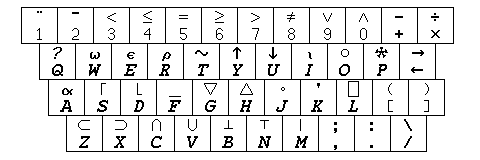
APL keyboard layout
Examples:
Hello, World!:
Example for versions Dyalog APL 13.1'Hello, World!'
Factorial:
Example for versions Dyalog APL 13.1The first line sets the index of the first element in the lists (in this case 0). The second line sets precision when printing numbers (must be greater than the length of the largest factorial).
The third line, if read in right-to-left direction, performs the following operations:
⍳17generates a list of 17 indices, starting with 0, i.e. 0 … 16.17 / ⊂'!='generates a list of 17 strings!=.⊂isencloseoperator which allows to manipulate strings as scalars instead of character arrays./is replication operator.!⍳17applies built-in monadic function!(factorial) to each element of the list.,is a dyadic operation which concatenates left and right arguments. After two concatenations the expression evaluates to0 1 2 3 4 ... 15 16 != != ... != 1 1 2 6 24 120 720 5040 40320 362880 ..., i.e. the list of numbers followed by the list of strings and the list of factorials.3 17⍴reshapes the list into a 3x17 matrix:┌→─┬──┬──┬──┬──┬───┬───┬────┬─────┬──────┬───────┬────────┬─────────┬──────────┬───────────┬─────────────┬──────────────┐ ↓0 │1 │2 │3 │4 │5 │6 │7 │8 │9 │10 │11 │12 │13 │14 │15 │16 │ ├~─┼~─┼~─┼~─┼~─┼~──┼~──┼~───┼~────┼~─────┼~──────┼~───────┼~────────┼~─────────┼~──────────┼~────────────┼~─────────────┤ │!=│!=│!=│!=│!=│!= │!= │!= │!= │!= │!= │!= │!= │!= │!= │!= │!= │ ├─→┼─→┼─→┼─→┼─→┼──→┼──→┼───→┼────→┼─────→┼──────→┼───────→┼────────→┼─────────→┼──────────→┼────────────→┼─────────────→┤ │1 │1 │2 │6 │24│120│720│5040│40320│362880│3628800│39916800│479001600│6227020800│87178291200│1307674368000│20922789888000│ └~─┴~─┴~─┴~─┴~─┴~──┴~──┴~───┴~────┴~─────┴~──────┴~───────┴~────────┴~─────────┴~──────────┴~────────────┴~─────────────┘finally,
⍉transposes this matrix so that each row has three elements — a number, a separator string and a factorial.
The program output looks like this:
     ┌→─┬──┬──────────────┐
     ↓0 │!=│1             │
     ├~─┼─→┼~─────────────┤
     │1 │!=│1             │
     ├~─┼─→┼~─────────────┤
     │2 │!=│2             │
     ├~─┼─→┼~─────────────┤
     [...25 lines of output ...]
     ├~─┼─→┼~─────────────┤
     │16│!=│20922789888000│
     └~─┴─→┴~─────────────┘
The matrix is displayed as a table with cell borders drawn, because it contains boxed strings.
⎕IO←0
⎕PP←18
⍉3 17⍴ (⍳17) , (17 / ⊂'!=') , !⍳17
Fibonacci numbers:
Example for versions Dyalog APL 13.1This example uses Binet’s formula implemented via an anonymous D-function. ⋄ is expression separator, so the function consists of two expressions evaluated in left-to-right order. The first one calculates golden ration and binds it to name phi. The second one calculates the value of the function (Fibonacci number) based on its right argument ⍵ (the index of the number). ⌈ rounds the number up.
Since the function is unary and is defined using scalar functions only, it can be applied to an array — in this case to an array of indices between 1 and 16, inclusive. This will result in an array of Fibonacci numbers:
1 1 2 3 5 8 13 21 34 55 89 144 233 377 610 987
{phi←(1+5*0.5)÷2 ⋄ ⌈((phi*⍵) - (1-phi)*⍵)÷5*0.5} 1+⍳16
Factorial:
Example for versions Dyalog APL 13.1This example calculates factorial of a number N by applying multiplication reduction to a list of numbers from 1 to N, inclusive (expression ×/1+⍳). The anonymous D-function applies this expression to its right argument and concatenates the result with the argument itself and a string separator. Note that in this case the string is not boxed. The function, in turn, is applied to a list of numbers from 0 to 16, written in a column, i.e. as a two-dimensional 17x1 array. Program output looks like this:
 ┌→───────────────────┐
 ↓0 != 1              │
 ├+──────────────────→┤
 │1 != 1              │
 ├+──────────────────→┤
 │2 != 2              │
 ├+──────────────────→┤
 [...25 lines of output ...]
 ├+──────────────────→┤
 │16 != 20922789888000│
 └+──────────────────→┘
⎕IO←0
⎕PP←18
{⍵, '!=', ×/1+⍳⍵}¨17 1⍴⍳17
Fibonacci numbers:
Example for versions Dyalog APL 13.1This example uses an anonymous D-function which calls itself recursively. The first expression of the function processes the case of the first two Fibonacci numbers, returning 1. The rest of them are processed by the second expression, which calls this very D-function (function ∇) for smaller indices of the numbers and sums them. Overall the first line of code associates the calculated array of numbers with name fib and outputs nothing.
The second line converts the array to required format: each element gets concatenated with a comma separator, all elements of the resulting array get concatenated with each other (,/), and the result is padded with .... The overall output of this line looks exactly as required:
1 , 1 , 2 , 3 , 5 , 8 , 13 , 21 , 34 , 55 , 89 , 144 , 233 , 377 , 610 , 987 , ...
fib←{⍵≤2:1 ⋄ (∇⍵-1)+∇⍵-2}¨1+⍳16
(⊃(,/{⍵, ', '}¨fib)),'...'
Quadratic equation:
Example for versions Dyalog APL 13.1This code defines a named D-function which accepts equation coefficients as a single argument (a three-element array) and returns equation solution. First the argument is split into separate coefficients (N⊃⍵ picks Nth element of the array) and they are assigned names. After this first coefficient and discriminant are checked — if one of them is zero, the function returns a special value. Finally, non-zero discriminant is processed with the same code regardless of its sign due to the fact that APL has built-in complex numbers datatype. A function call
solve 1 0 2
will return:
0J1.4142135623730951 0J¯1.4142135623730951
(J is a separator between real and imaginary parts of the number, and ¯ — is a “high” minus, used for input/output of negative numbers).
Note that this code is not typical for APL due to conditional branching use as well as limiting possible arguments to a one-dimensional array of three elements.
solve←{A←0⊃⍵ ⋄ B←1⊃⍵ ⋄ C←2⊃⍵ ⋄ A=0:'Not a quadratic equation.' ⋄ D←(B*2)-4×A×C ⋄ D=0:-0.5×B÷A ⋄ ((-B-D*0.5), -B+D*0.5)×0.5÷A}
Comments
]]>blog comments powered by Disqus
]]>